CryoFM: A Flow-based Foundation Model<br/>for Cryo-EM Densities

TL;DR.
CryoFM is a flow matching based foundation model that learns a generative prior over biomolecular density maps. It enables flexible posterior sampling for diverse cryo-EM and cryo-ET tasks without fine-tuning, achieving state-of-the-art results.

📄OpenReview·📄arXiv·💻Code·📖User Guides·📊Data list

Overview

Cryo-electron microscopy (cryo-EM) is a powerful technique in structural biology and drug discovery, enabling the study of biomolecules at high resolution. Significant advancements by structural biologists using cryo-EM have led to the production of around 50k protein density maps at various resolutions on EMDB.¹ However, cryo-EM data processing algorithms have yet to fully benefit from our knowledge of biomolecular density maps, with only a few recent models being data-driven but limited to specific tasks. In this study, we present cryoFM, a foundation model designed as a generative model, learning the distribution of high-quality density maps and generalizing effectively to downstream tasks. Built on flow matching, cryoFM is trained to accurately capture the prior distribution of biomolecular density maps. Furthermore, we introduce a flow posterior sampling method that leverages cryoFM as a flexible prior for several downstream tasks in cryo-EM and cryo-electron tomography (cryo-ET) without the need for fine-tuning, achieving state-of-the-art performance on most tasks and demonstrating its potential as a foundational model for broader applications in these fields.

What cryoFM enables.

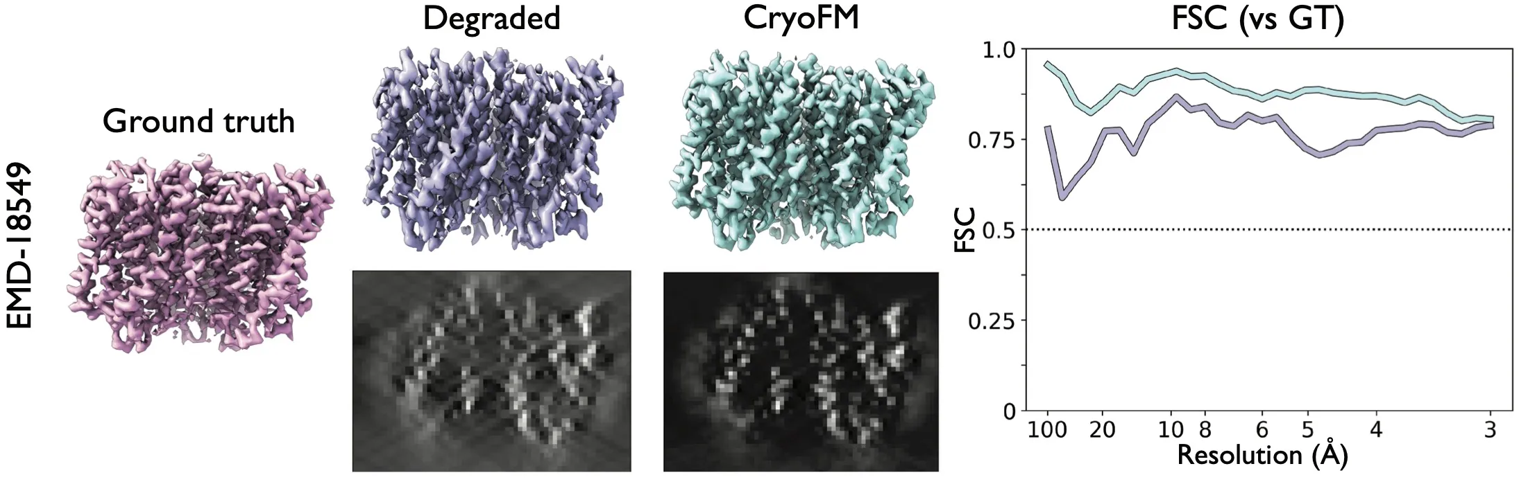
In the training stage, cryoFM learns a vector field $\mathbf{v}_t(\mathbf{x}_t)$ , whose corresponding probability flow generates the data distribution $p_0(\mathbf{x}_0)$ of high-quality protein densities. In the inference stage, given a degraded observation $\mathbf{y}$ , a likelihood term $p_t(\mathbf{y} \mid \mathbf{x}_t)$ is incorporated to convert the unconditional vector field $\mathbf{v}_t(\mathbf{x}_t)$ to a conditional one $\mathbf{v}_t(\mathbf{x}_t \mid \mathbf{y})$ , so that we can sample from the posterior distribution $p_0(\mathbf{x}_0 \mid \mathbf{y})$ . This enables signal restoration of the density map, resulting in improved resolution of the alpha helices in the shown case.

Key Contributions

Density-space foundation model: learns a generalizable prior over macromolecular density distributions.
Bayesian, controllable inference: enables posterior sampling by combining the learned prior with a likelihood function defined by physics-based forward operators.

Method at a Glance

Flow matching prior

CryoFM employs flow matching to learn a generative prior over biomolecular density maps, enabling flexible posterior sampling for diverse downstream tasks without fine-tuning. Specifically:

Data: 3D density patches (e.g., $64^3$ ), unsupervised pre-training on curated EMDB deposited maps
Model: 3D HDiT² predicting velocity for ODE-based generation

The following picture shows cryoFM’s architecture. The side length $D$ of the input $\mathbf{x}_t$ undergoes dimension reduction through down-sampling layers and is then expanded back to its original size. To minimize computational cost near the input and output, the model employs neighborhood attention (NA). Neighborhood attention only attend to a localized area, whereas global attention (GA) calculates attention across all positions.

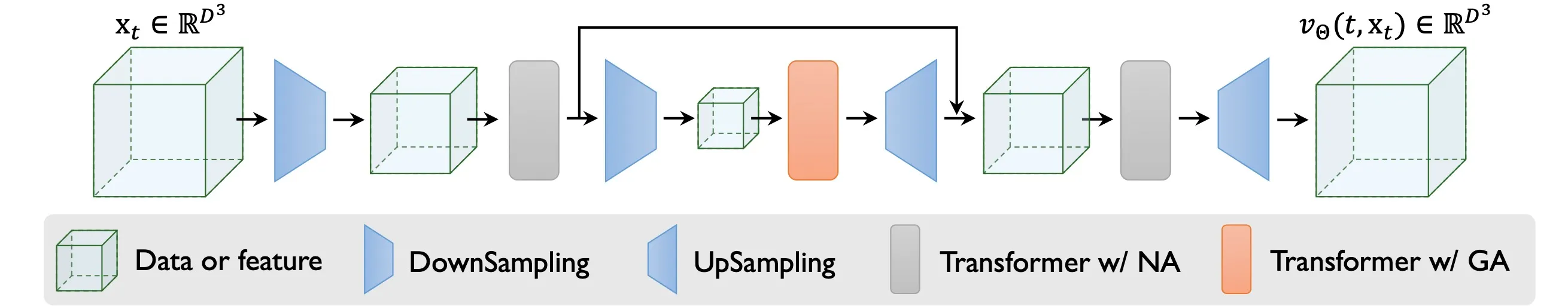
CryoFM’s architecture.

CryoFM adopts the network architecture proposed in the HDiT paper². The attention mechanism in CryoFM employs two complementary strategies: neighborhood attention (NA) and global attention (GA). NA focuses on local spatial relationships within a constrained region, reducing computational complexity while maintaining fine-grained local features. In contrast, GA captures long-range dependencies across the entire volume, enabling the model to integrate global structural information. The following figure illustrates the QKV (Query, Key, Value) structure of both attention mechanisms, highlighting their distinct computational patterns.

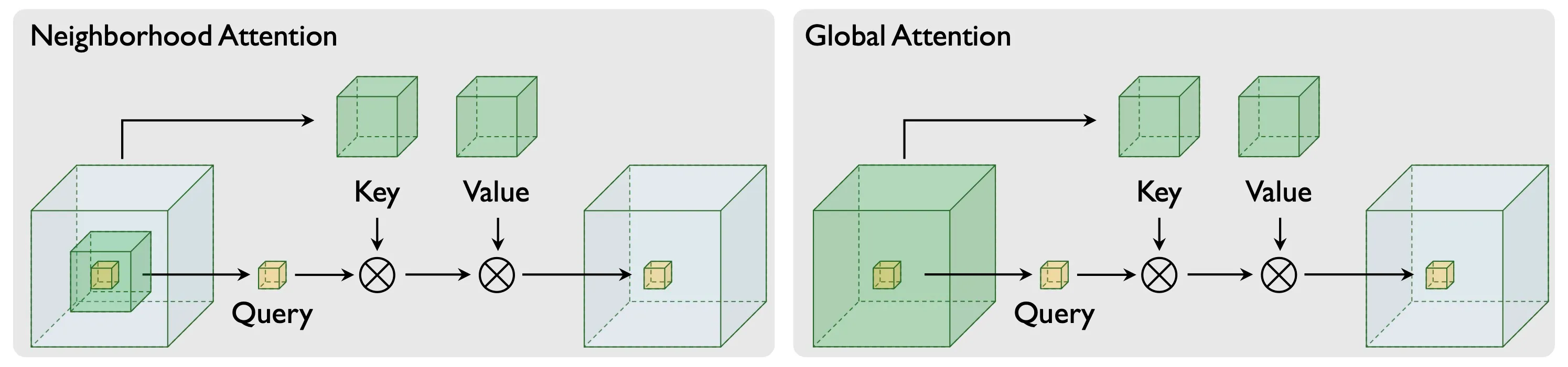
Illustration of QKV structure of neighborhood attention (NA) and global attention (GA).

Flow Posterior Sampling

Given a degraded observation $\mathbf{y}$ , we recover the clean signal $\mathbf{x}_0$ by combining the learned prior with the likelihood function through the following algorithm:

Algorithm 1: Flow Posterior Sampling

Require:

v_\Theta

: pretrained vector field

[0, 1] \times \mathbb{R}^n \to \mathbb{R}^n

A

: forward operator

\mathbb{R}^n \to \mathbb{R}^m

\mathbf{y}

: observation

\in \mathbb{R}^m

N

: number of steps

\lambda_{\max}

: maximum step size

Ensure:

\mathbf{x}_0

: recovered signal

\Delta t \leftarrow 1 / N

\mathbf{x}_1 \leftarrow \mathcal{N}(0, I)

// Initialize from standard normal

for

t \in [1, 1-\Delta t, 1-2\Delta t, \ldots, \Delta t]

\mathbf{x}'_{t-\Delta t} \leftarrow \mathbf{x}_t - \Delta t \cdot v_\Theta(t, \mathbf{x}_t)

l(\mathbf{x}_t) \leftarrow \|\mathbf{y} - A \hat{\mathbf{x}}_0(\mathbf{x}_t)\|^2

// Likelihood loss

\mathbf{g} \leftarrow \nabla_{\mathbf{x}_t} l(\mathbf{x}_t) / \|\nabla_{\mathbf{x}_t} l(\mathbf{x}_t)\|_2

// Normalize gradient for numerical stability

\lambda'_t \leftarrow \min\{\lambda_{\max}, t / (1 - t)\}

// Prevent the weighting term from being too large

\mathbf{x}_{t-\Delta t} \leftarrow \mathbf{x}'_{t-\Delta t} - \lambda'_t \mathbf{g}

end for

10:

return

\mathbf{x}_0

The algorithm iteratively refines the signal by:

Following the learned prior through the vector field $v_Θ$
Incorporating the likelihood constraint via gradient guidance
Using adaptive step sizes to ensure numerical stability

We demonstrate the effectiveness of our method on 4 synthetic tasks: Spectral noise de-noising, Anisotropic noise de-noising, Missing wedge in-painting, Ab initio modeling.

Results on 4 tasks

Spectral noise de-noising

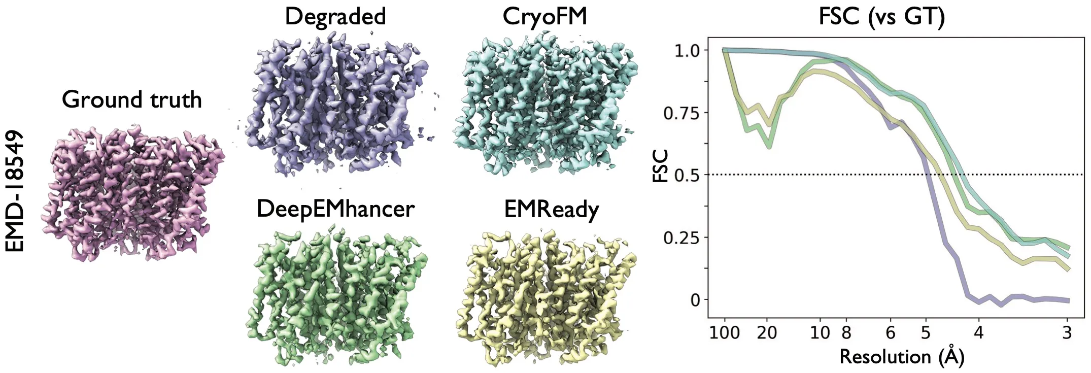
Result of the spectral noise denoising task. Two density maps from EMDB were added spectral noise so that the estimated resolution is 4.3 $\AA$ The degraded density maps (results after applying the forward model) were filtered by relion_postprocess for visual clarity.

Anisotropic noise de-noising

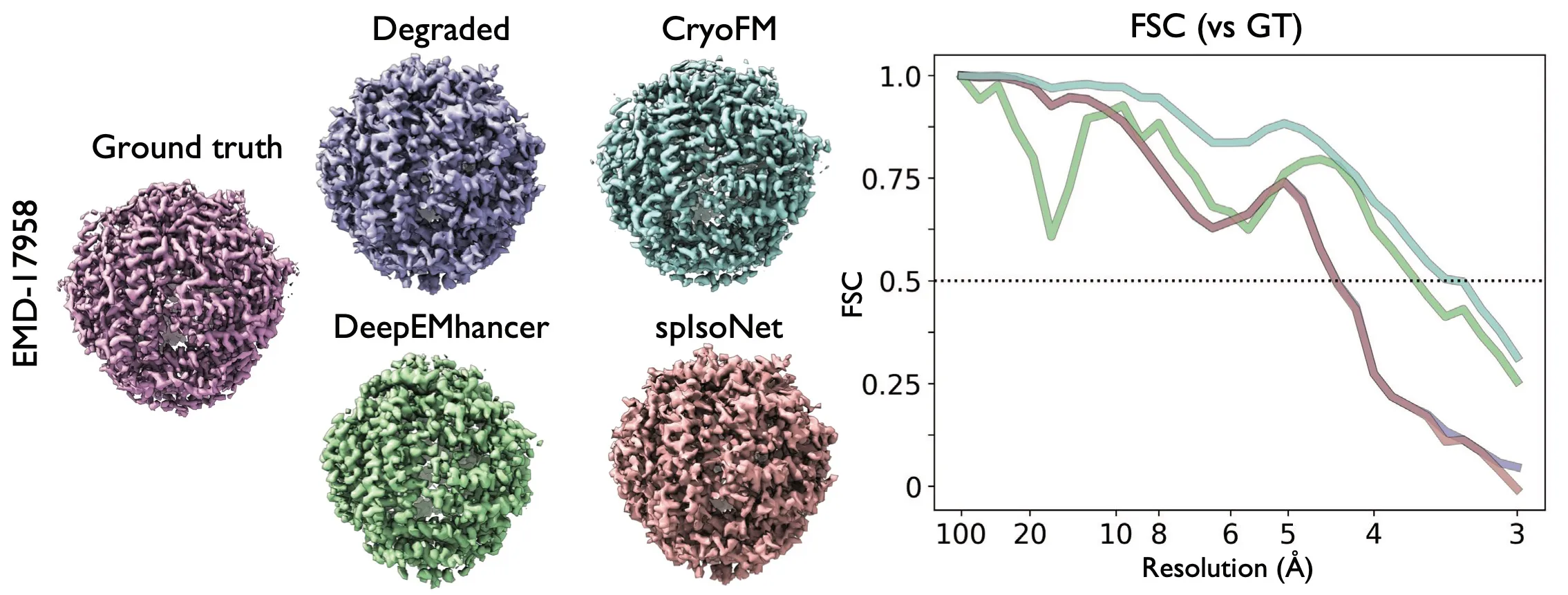
Result of the anisotropic noise denoising task. Two density maps from EMDB are added anisotropic spectral noise that the estimated resolution is 4.38 $\AA$ . The degraded density maps are filtered by relion_postprocess for visual clarity.

Missing wedge in-painting

Result of the missing wedge restoration task. Two maps from EMDB are masked in Fourier space to simulate the missing wedge effect in cryo-ET. The central slices through the maps are also shown.

Ab initio modeling

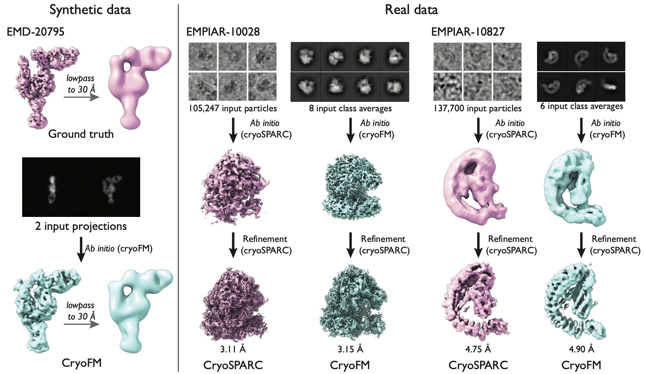
Result of the ab initio modeling task. One synthetic data and two real data are shown.

Citation

If you find CryoFM helpful, please cite:

@inproceedings{
zhou2025cryofm,
title={Cryo{FM}: A Flow-based Foundation Model for Cryo-{EM} Densities},
author={Yi Zhou and Yilai Li and Jing Yuan and Quanquan Gu},
booktitle={The Thirteenth International Conference on Learning Representations},
year={2025},
url={https://openreview.net/forum?id=T4sMzjy7fO}
}

As of 17 December 2025, the Electron Microscopy Data Bank (EMDB) lists 52,575 cryo-EM map entries; see the official statistics at EMDB. ↩
Hourglass Diffusion Transformer (HDiT) is introduced in “Scalable High-Resolution Pixel-Space Image Synthesis with Hourglass Diffusion Transformers” by Crowson et al., 2024; see arXiv:2401.11605. ↩ ↩²